Simple Linear Regression A WebQuest for exploring relationships between variables using simple linear regression. 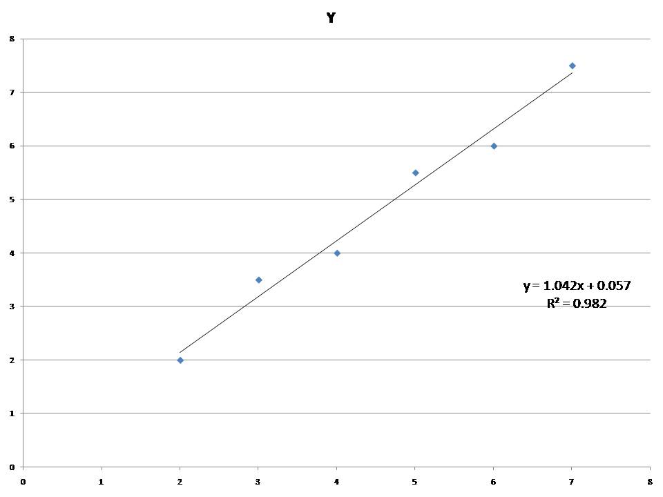Designed by Joseph A. Snider, 2009  Introduction Task Process Evaluation Conclusion Credits Introduction Simple linear regression is a statistical method used to show the relationship between two variables (Weisberg, 2005). You start with pairs of values called X and Y. These can be any numerical values. The goal is to see if there is a relationship between X and Y and to determine if it is a strong relationship. Simple Linear Regression is useful in a wide set of applications and industries, and since it is simple to use, the method is a good starting point to analyze existing data and then predict Y values for any X. The only rule of thumb is to pick X values within your minimum and maximum. Using values outside of your minimum and maximum X is called extrapolation, and can yield bad results. The X value is called the independent variable and the Y value is called the dependent variable. In common language, the Y values depend on what X values you choose. While you can determine if a relationship exists with Simple Linear Regression, the relationship is not necessarily a cause and effect relationship. It takes more study to determine cause and effect relationships. The equation that best represents your data as a line on the chart is called the Simple Linear Regression Equation. It takes the form of Y = slope times X plus the y-intercept. The slope is defined as the change in Y when X changes 1 unit of whatever you are measuring. The y-intercept is the Y value when X has a value of zero. In the chart above, 1.042 is the value for the slope and .057 is the value for the y-intercept. The slope and y-intercept are the two values we need to create the linear regression equation. The nice thing about Microsoft Excel (R) is that it can calculate the values for you while producing the chart. The R squared value is defined as the coefficient of determination. R squared shows the amount of variation in Y that can be determined from the variation in X. If the value is nearer to 1, it shows a strong relationship between X values and Y values. If the value is nearer to 0 (Zero), it shows a weak relationship between X values and Y values. (Bewick, Cheek, & Ball, 2003).   The Task In this lesson, you will be able to use Microsoft Excel (R) to: 1. Enter raw data into a spreadsheet 2. Chart raw data as a scatter plot chart 3. Create a trend line showing the simple linear regression equation 4. Predict a Y value for a given X value In order to master the skill, you can run the video and audio tutorial lesson as many times as you need to. The Process First you'll run the spreadsheet tutorial... Now try what you learned on this set of X and Y pairs of values. - Enter the following data into a blank spreadsheet - Create a scatterplot chart from them - Create a trend line showing the simple linear regression equation - Predict a Y value when X = 2004.2 X Y 2001.5 24.6 2002.9 33.2 2003.2 44.8 2004.3 55.2 2005.6 66.4 Check your results against Y = 10.63 times X - 21264 as the simple regression equation and the predicted Y value = 40.646 when X = 2004.2 If your results are different, you might be using a different number of decimal values in your calculation or the results. If the numbers are way off, run the tutorial again to figure out how to run the process. In a normal course, this is a good opportunity to have a student turn in results for a grade, but as research, just compare your results to make sure you performed the function correctly. Now try what you learned on this set of X and Y pairs of values. - Enter the following data into a blank spreadsheet - Create a scatterplot chart from them, - Create a trend line showing the simple linear regression equation - Predict a Y value when X=2.46 X Y 1 6.57 2 5.22 3 4.17 4 3.33 5 2.05 Check your results against Y = -1.093 times X + 7.547 as the simple regression equation and the predicted Y value = 4.858 when X = 2.46 If your results are different, it could be the number of decimal places. If way off, run the tutorial again to figure out how to run the process. In a normal course, this is a good opportunity to have a student turn in results for a grade, but as research, just compare your results to make sure you performed the function correctly. Now try what you learned on this set of X and Y pairs of values. - Enter the following data into a blank spreadsheet - Create a scatterplot chart from them - Create a trend line showing the simple linear regression equation - Predict a Y value when X=20.4 X Y 10 2 20 3 30 4 40 5 50 6 Check your results against Y = .1 times X + 1 as the simple regression equation and the predicted Y value = 3.04 when X = 20.4 If your results are different, it could be the number of decimal places. If way off, run the tutorial again to figure out how to run the process. In a normal course, this is a good opportunity to have a student turn in results for a grade, but as research, just compare your results to make sure you performed the function correctly. Now try what you learned on this set of X and Y pairs of values. - Enter the following data into a blank spreadsheet - Create a scatterplot chart from them - Create a trend line showing the simple linear regression equation - Predict a Y value when X=294 X Y 100 -217 200 -304 300 -414 400 -566 500 -601 Check your results against Y = -1.03 times X - 111.4 as the simple regression equation and the predicted Y value = -414.22 when X = 294 If your results are different, it could be the number of decimal places. If way off, run the tutorial again to figure out how to run the process. In a normal course, this is a good opportunity to have a student turn in results for a grade, but as research, just compare your results to make sure you performed the function correctly. Evaluation There is a maximum of 8 points for this lesson. Beginning 1 Developing 2 Accomplished 3 Exemplary 4 Score   Stated Objective or Performance For zero or 1 of the above practice problems, the Student accurately can derive the Simple Linear Regression equation using Microsoft Excel (R). For 2 of the above practice problems, the Student accurately can derive the Simple Linear Regression equation using Microsoft Excel (R). For 3 of the above practice problems, the Student accurately can derive the Simple Linear Regression equation using Microsoft Excel (R). For 4 of the above practice problems, the Student accurately can derive the Simple Linear Regression equation using Microsoft Excel (R). 1-4   Stated Objective or Performance For zero or 1 of the above practice problems, the Student accurately can predict the correct Y value for the given X value using Microsoft Excel (R). For 2 of the above practice problems, the Student accurately can predict the correct Y value for the given X value using Microsoft Excel (R). For 3 of the above practice problems, the Student accurately can predict the correct Y value for the given X value using Microsoft Excel (R). For 4 of the above practice problems, the Student accurately can predict the correct Y value for the given X value using Microsoft Excel (R). 1-4 Total--> 2-8 Conclusion To master the skill of performing Simple Linear Regression, a person needs to be able to derive the Simple Linear Regression equation and to be able to predict a Y value for a given X value. Microsoft Excel (R) is used in this skills training to make the calculations quick and easy. If you reached at least a score of 6 from the rubric above, you are ready to move to the next stage. If not, repeat the tutorial and try again. Credits & References The image and data used in this WebQuest are original material. The concepts regarding Simple Linear Regression can also be found in following references: Teach Yourself Statistics (2009). AP Statistics tutorial: Least squares linear regression. Retrieved from http://stattrek.com/AP-Statistics-1/Regression.aspx CAUSEweb (2009). The Consortium to Advance Undergraduate Statistics Education. Retrieved from http://www.causeweb.org Bewick, V., Cheek, L., & Ball, J. (2003). Statistics review 7: Correlation and regression. Retrieved from http://ccforum.com/content/7/6/451 Weisberg, S. (2005). Applied Linear Regression, 3rd Ed. published by Wiley/Interscience in 2005 (ISBN 0-471-66379-4). For important guidelines on how to teach statistics for college level students, see the following reference: GAISE (2005). The American Statistical Association Web site Guidelines for Assessment and Instruction in Statistics Education (GAISE) College report. Retrieved from http://www.amstat.org/education/GAISE